- ERS
- Mission
- Radar Courses
- Radar Course 3
ERS Radar Course 3
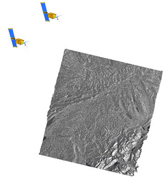
1. Independence of solar illumination
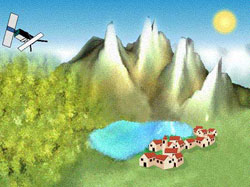
SAR is an active system.
It illuminates the Earth surface and measures the reflected signal. Therefore, images can be acquired day and night, completely independent of solar illumination, which is particularly important in high latitudes (polar night).
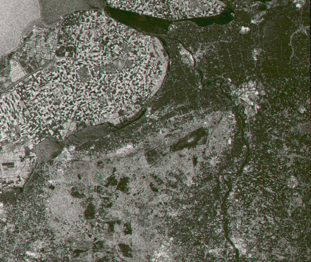
This SAR image was acquired by ERS-1 on 2 August 1991 over the Netherlands, local time 23:40.
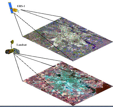
2. Independence of cloud coverage
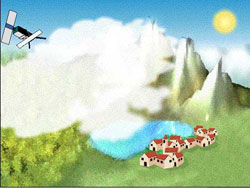
The microwaves emitted and received by ERS SAR are at much longer wavelengths (5.6 cm) than optical or infrared waves. Therefore, microwaves easily penetrate clouds, and images can be acquired independently of the current weather conditions.
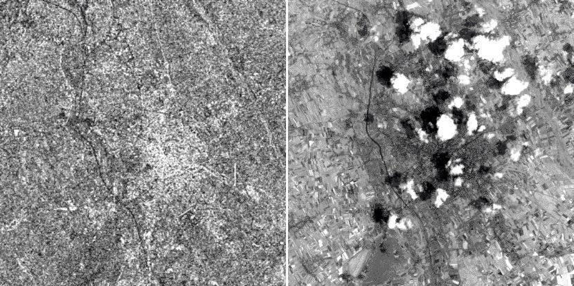
These images were acquired over the city of Udine (I), by ERS-1 on 4 July 1993 at 09:59 (GMT) and Landsat-5 on the same date at 09:14 (GMT) respectively. The clouds that are clearly visible in the optical image, do not appear in the SAR image.
3. Control of emitted electromagnetic radiation
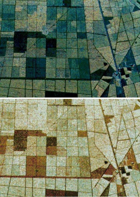
Because an imaging radar is an active system, the properties of the transmitted and received electromagnetic radiation (power, frequency, polarization) can be optimised according to mission specification goals.
The top part of the image shows a three band combination (P-Band-->RED, L-Band-->GREEN and C-Band-->BLUE) for JPL aircraft SAR overfly over Landes (F) during the MAESTRO-1 campaign. On the bottom side, a multipolarization combination (HH -->RED, VV-->GREEN and HV-->BLUE) shows different details of the same site.
4. Control of imaging geometry
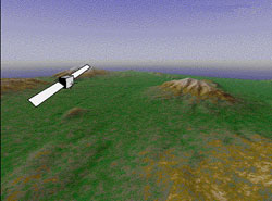
Because an imaging radar is an active system, the geometric configuration for illuminating the terrain (altitude of aircraft/spacecraft depression angle) can be optimised according to mission specification goals.
5. Access to different parameters compared to optical systems
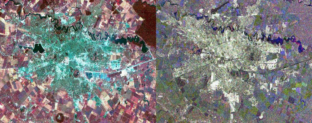
Images provided by optical sensors contain information about the surface layer of the imaged objects (i.e. colour), while microwave images provide information about the geometric and dielectric properties of the surface or volume studied (i.e., roughness).
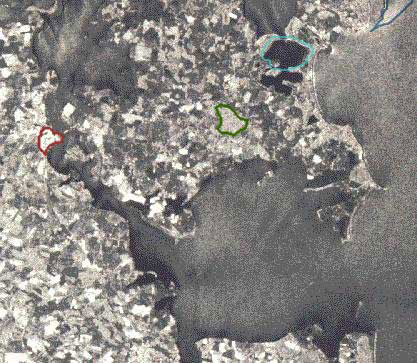
These images were acquired over the city of Bucharest (R), by ERS-1 and Landsat-5 respectively. The city has a star-shaped urban structure, with a historical centre from which the urban area extends along the main road.
In the centre of the city, the presidential palace can be seen, and to the right even the main entry is visible.
The main avenues form three concentric rings around the centre. The national airport is located in the north. The Dimbovita river, a tributary of the Danube, crosses the northern part of the city, and has meanders, partly filled by an artificial lake. Other lakes are visible in the center and in the lower part of the image. The circular zone in the South is a forested area, with a large building in the centre.
The vegetation visible in the image is an agricultural area, mainly corn fields. In the north, large zones essentially covered by trees can be observed.
The SAR image is a multi-temporal composition of three images (3/07/92, 25/11/92, 30/12/92), the urban area is well imaged and the density of the built-up area can be assessed by the strength of the backscattered signal.
In contrast to the optical image, highways, large roads and avenues are presented as dark lines. This is also true for the runways on airports, because of the smooth surface. Bridges and railways on the contrary are imaged mostly very brightly due to the dielectric property of metal.
The different colours of the agricultural fields depend on the changes in surface roughness occurred between the acquisition dates.
Data acquired in spring and summer is used to identify the crop type, a methodology similar to the one applied with optical data.
However, it has been reported that data acquired in the winter is also of great interest, since it reveals the type of field labour performed, which is often typical of the preparation of the fields for certain crops. The data helps to assess certain crop types and estimate their surfaces very early in the year.
It is obvious that such data application must be based on good knowledge of the time and type of field preparation. Initially sufficient ground survey needs to be available.
6. Electromagnetic Spectrum
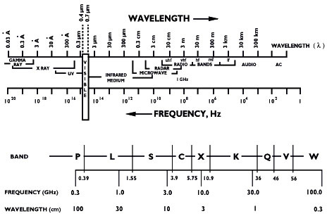
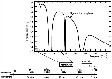
The useful part of the electromagnetic spectrum is shown in the upper part of this figure. Obviously, it covers many decades in frequency (or wavelength).
The lowest frequencies (longest wavelengths) constitute the radio spectrum. Parts of the radio spectrum are used for radar and passive detection.
Above the radio-frequency spectrum lies the infrared spectrum, followed by the visible range, which is quite narrow. Multispectral scanners are operated in the visible and infrared regions of the spectrum, and are used extensively as remote sensing tools for a wide variety of applications. Above the visible spectrum lies the ultraviolet spectrum and, overlapping it, the X-ray spectrum. Finally, at the highest frequencies are the gamma rays, which are sometimes used in remote sensing; for example, in the determination of the presence of moisture due to the absorption of gamma rays by moisture.
The lower part of the figure illustrates the microwave portion of the spectrum. The portion shown extends from 0.3 to 100 GHz.
Frequencies down to 0.1 Hz are used in magnetotelluric sensing of the structure of the Earth, and frequencies in the range between 0.1 Hz and 1 kHz sometimes are used both for communication with submarines (at least this is a proposed use) and for certain kinds of sensing of the ionosphere and the Earth's crust.
These frequencies certainly are far from the microwave range. Letter designations are shown for decade regions of the spectrum above the frequency chart. These designations have been adopted internationally by the International Telecommunication Union (ITU).
The very-low-frequency (VLF) region from 3 to 30 kHz is used for both submarine communication and for the Omega navigation system. The Omega system might be considered to be a form of radar - but for use in position location, not for remote sensing.
The low-frequency (LF) region, from 30 to 300 kHz, is used for some forms of communication, and for the Loran C position-location system. At the high end of this range are some radio beacons and weather broadcast stations used in air navigation, although in most areas of the world these are being phased out.
The medium-frequency (MF) region from 300 to 3000 kHz contains the standard broadcast band from 500 to 1500 kHz, with some marine communications remaining below the band and various communication services above it. The original Loran A system also was just above the broadcast band at about 1.8 MHz. This, too, is a form of radar system, but it is being phased out.
The high-frequency (HF) from 3 to 30 MHz is used primarily for long-distance communication and short-wave broadcasting over long distances, because this is the region most affected by reflections from the ionosphere and least affected by absorption in the ionosphere. Because of the use of ionosphere reflection in this region, some radar systems are operated in the HF region. One application is an ionospherically reflected long-distance radar for measuring properties of ocean waves from a shore station.
The very-high-frequency (VHF) region from 30 to 300 MHz is used primarily for television and FM broadcasting over line-of-sight distances and also for communication with aircraft and other vehicles. However, some radars intended for remote sensing have been built in this frequency range, although none are used operationally. Some of the early radio-astronomy work also was done in this range, but radiometers for observing the Earth have not ordinarily operated at such long wavelengths because of the difficulty of getting narrow antenna beams with reasonable-size antennas.
The ultra-high-frequency (UHF) region from 300 to 3000 MHz is extensively populated with radars, although part of it is used for television broadcasting and for mobile communications with aircraft and surface vehicles. The radars in this region of the spectrum are normally used for aircraft detection and tracking, but the lower frequency imaging radars such as that on Seasat and the JPL and ERIM experimental SARs also are found in this frequency range.
Microwave radiometers are often found at 1.665 GHz, where nitric oxide (NO) has a resonance. Extensive radio-astronomy research is done using these resonances, and the availability of a channel clear of transmitter radiation is essential. The passive microwave radiometers thus can take advantage of this radio-astronomy frequency allocation.
The super-high-frequency (SHF) ranges from 3 to 30 GHz is used for most of the remote sensing systems, but has many other applications as well. The remote sensing radars are concentrated in the region between 9 and 10 GHz and around 14 to 16 GHz.
Satellite communications use bands near 4 and 6 GHz and between 11 and 13 GHz as well as some higher frequencies. Point-to-point radio communications and various kinds of ground-based radar and ship radar are scattered throughout the range, as are aircraft navigation systems. Because of a water-vapour absorption near 22 GHz (see this figure), that part of the SHF region near 22 GHz is used almost exclusively for radiometric observations of the atmosphere. Additionally, remote sensing radiometers operate at several points within the SHF range, primarily within the radio-astronomy allocations centred at 4.995, 10.69, 15.375, and 19.35 GHz.
Most of the extremely-high-frequency (EHF) range from 30 to 300 GHz is used less extensively, although the atmospheric-window region between 30 and 40 GHz is rather widely used and applications in the neighbourhood of 90 to 100 GHz are increasing.
Because of the strong oxygen absorption in the neighbourhood of 60 GHz, frequencies in the 40-70 GHz region are not used by active systems. However, multi-frequency radiometers operating in the 50-60 GHz range are used for retrieving the atmospheric temperature profiles from radiometric observations.
Radars are operated for remote sensing in the 32-36 GHz region, and some military imaging radars are around 95 GHz. Radio-astronomy bands exist at 31.4, 37, and 89 GHz, and these are, of course, used by microwave radiometers for remote sensing as well.
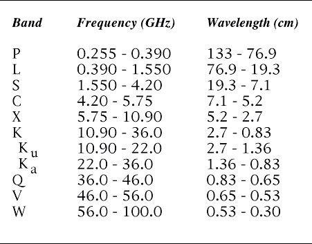
The microwave spectrum itself is illustrated in this table. No firm definition exists for the microwave region, but a reasonable convention is that it extends throughout the internationally designed UHF, SHF, and EHF bands from 0.3 to 300 GHz (1 m to 1 mm in wavelength). Numerous schemes of letter designation for bands in the microwave region exist, and they are indicated in the figure.
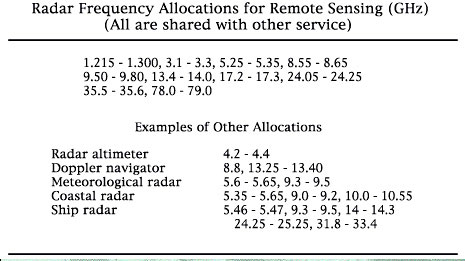
Radars may be found in all of the bands, with the possible exception of the Q- and V-bands, with most remote sensing radars at K-band or lower frequencies. Frequency allocations are made on an international basis at periodic but infrequent World Administrative Radio Conferences, which classify radars as "radiolocation stations". Several of the radiolocation allocations of the 1979 WARC list radar for Earth observation as a secondary service to other radars, and some permit such use as a primary service. This table lists these allocations along with some selected non-remote sensing allocations.
Sharing between radar remote sensing systems and other radars is usually not permitted. Thus, the designer of a remote sensing radar system cannot simply choose an optimum frequency and use it.
7. Radar principles
Radar sensors are usually divided into two groups according to their modes of operation. Active sensors are those that provide their own illumination and therefore contain a transmitter and a receiver, while passive sensors are simply receivers that measure the radiation emanating from the scene under observation.
Active systems:
- Radar imaging systems (Radar = RAdio Detection And Ranging)
- Scatterometers
- Altimeters
Passive systems:
- Microwave radiometers
We are interested in radar imaging systems. The basic principle of a radar is transmission and reception of pulses. Short (microsecond) high energy pulses are emitted and the returning echoes recorded, providing information on:
- Magnitude
- Phase
- Time interval between pulse emission and return from the object
- Polarization
- Doppler frequency
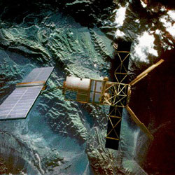
The same antenna is often used for transmission and reception. This image presents the basic elements of an imaging radar system.
The two types of imaging radars most commonly used are:
- RAR --> Real Aperture Radar
- SAR --> Synthetic Aperture Radar
Real Aperture radars are often called SLAR (Side Looking Airborne Radar). Both Real Aperture and Synthetic Aperture Radar are side-looking systems with an illumination direction usually perpendicular to the flight line.
The difference lies in the resolution of the along-track, or azimuth direction. Real Aperture Radars have azimuth resolution determined by the antenna beamwidth, so that it is proportional to the distance between the radar and the target (slant-range).
Synthetic Aperture Radar uses signal processing to synthesise an aperture that is hundreds of times longer than the actual antenna by operating on a sequence of signals recorded in the system memory.
These systems have azimuth resolution (along-track resolution) that is independent of the distance between the antenna and the target.
The nominal azimuth resolution for a SAR is half of the real antenna size, although larger resolution may be selected so that other aspects of image quality may be improved.
Generally, depending on the processing, resolutions achieved are of the order of 1-2 metres for airborne radars and 5-50 metres for spaceborne radars.
8. Side-looking radars

Most imaging radars used for remote sensing are side-looking airborne radars (SLARs). The antenna points to the side with a beam that is wide vertically and narrow horizontally. The image is produced by motion of the aircraft past the area being covered.
A short pulse is transmitted from the airborne radar, when the pulse strikes a target of some kind, a signal returns to the aircraft. The time delay associated with this received signal, as with other pulse radars, gives the distance between target and radar.
When a single pulse is transmitted, the return signal can be displayed on an oscilloscope; however, this does not allow the production of an image. Hence, in the imaging radar, the signal return is used to modulate the intensity of the beam on the oscilloscope, rather than to display it vertically in proportion to the signal strength.
Thus, a single intensity-modulated line appears on the oscilloscope, and is transferred by a lens to a film. The film is in the form of a strip that moves synchronously with the motion of the aircraft, so that as the aircraft moves forward the film also moves.
When the aircraft has moved one beamwidth forward, the return signals come from a different strip on the ground. These signals intensity-modulate the line on the cathode-ray tube and produce a different image on a line on the film adjacent to the original line. As the aircraft moves forward, a series of these lines is imaged onto the film, and the result is a two-dimensional picture of the radar return from the surface.
The speed of the film is adjusted so that the scales of the image in the directions perpendicular to and along the flight track are maintained as nearly identical to each other as possible. Because the cross-track dimension in the image is determined by a time measurement, and the time measurement is associated with the direct distance (slant range) from the radar to the point on the surface, the map is distorted somewhat by the difference between the slant range and the horizontal distance, or ground range.
In some radar systems, this distortion is removed by making the sweep on the cathode-ray tube nonlinear, so that the points are mapped in their proper ground range relationship. This, however, only applies exactly if the points all lie in a plane surface, and this modification can result in excessive distortion in mountainous areas.
Side-looking airborne radars normally are divided into two groups: the real-aperture systems that depend on the beamwidth determined by the actual antenna, and the synthetic aperture systems that depend upon signal processing to achieve a much narrower beamwidth in the along-track direction than that attainable with the real antenna.
The customary nomenclature used is "SLAR" for the real-aperture system and "SAR" for the synthetic aperture system, although the latter is also a side-looking airborne (or spaceborne) radar.
9. Real Aperture Radar (RAR)
A narrow beam of energy is directed perpendicularly to the flight path of the carrier platform (aircraft or spacecraft). A pulse of energy is transmitted from the radar antenna, and the relative intensity of the reflections is used to produce an image of a narrow strip of terrain.
Reflections from larger ranges arrive back at the radar after proportionately larger time, which becomes the range direction in the image. When the next pulse is transmitted, the radar will have moved forward a small distance and a slightly different strip of terrain will be imaged.
These sequential strips of terrain will then be recorded side by side to build up the azimuth direction. The image consists of the two dimensional data array.
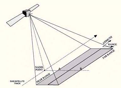
In this figure, the strip of terrain to be imaged is from point A to point B. Point A being nearest to the nadir point is said to lie at near range and point B, being furthest, is said to lie at far range.
The distance between A and B defines the swath width. The distance between any point within the swath and the radar is called its slant range.
Ground range for any point within the swath is its distance from the nadir point (point on the ground directly underneath the radar).
10. Real Aperture Radar: Range resolution
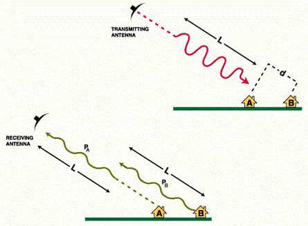
For the radar to be able to distinguish two closely spaced elements, their echoes must necessarily be received at different times.
In the upper part of the figure, the pulse of length L is approaching buildings A and B. The slant range distance between the two buildings is d.
Since the radar pulse must travel two ways, the two buildings lead to two distinguished echoes if:
d > L/2
The part of the pulse backscattered by building A is PA, and the part of the pulse backscattered by building B is PB.
It appears in the lower part of the figure that to reach the target and come back, PB has covered an extra distance 2d, and thus is at a slightly shorter distance than L behind PA.
Because of this, the end of PA and the beginning of PB overlap when they reach the antenna. As a consequence, they are imaged as one single large target which extends from A to B.
If the slant range distance between A and B were slightly higher than L/2, the two pulses would not overlap and the two signals would be recorded separately.
Range resolution (across track resolution) is approximately equal to L/2, i.e. half the pulse length.
Ground range resolution is:
where:
c speed of light
t pulse duration
q incidence angle
Incidence angle is the angle between the vertical to the terrain and the line going from the antenna to the object.
To improve range resolution, radar pulses should be as short as possible. However, it is also necessary for the pulses to transmit enough energy to enable the detection of the reflected signals.
If the pulse is shortened, its amplitude must be increased to keep the same total energy in the pulse.
One limitation is the fact that the equipment required to transmit a very short, high-energy pulse is difficult to build.
For this reason, most long range radar systems use the "chirp" approach which is an alternative method of pulse compression by frequency modulation.
In the case of the chirp technique, instead of a short pulse with a constant frequency, a long pulse is emitted with a modulated frequency.
The frequency modulation must be processed after reception to focus the pulse to a much shorter value. For the user, the result is the same as if a very short pulse had been used throughout the system.
11. Real Aperture Radar: Azimuth resolution
Azimuth resolution describes the ability of an imaging radar to separate two closely spaced scatterers in the direction parallel to the motion vector of the sensor.
In the image when two objects are in the radar beam simultaneously, for almost all pulses, they both cause reflections, and their echoes will be received at the same time.
However, the reflected echo from the third object will not be received until the radar moves forward. When the third object is illuminated, the first two objects are no longer illuminated, thus the echo from this object will be recorded separately.
For a real aperture radar, two targets in the azimuth or along-track resolution can be separated only if the distance between them is larger than the radar beamwidth. Hence the beamwidth is taken as the azimuth resolution depending also slant-range distance to the target for these systems.
For all types of radars, the beamwidth is a constant angular value with range. For a diffraction limited system, for a given wavelength l, the azimuth beamwidth b depends on the physical length dH of the antenna in the horizontal direction according to:
b = l/dH
For example, to obtain a beamwidth of 10 milliradians using 50 millimetres wavelength, it would be necessary to use an antenna 5 metres long. The real aperture azimuth resolution is given by:
raz = R* b
where:
raz azimuth resolution
R slant range
For example for a Real Aperture Radar of beamwidth 10 milliradians, at a slant range R equal to 700 kilometres, the azimuth resolution raz will be:
raz = 700 x 0.01
raz = 7 km
Real Aperture Radars do not provide fine resolution from orbital altitudes, although they have been built and operated successfully (for example COSMOS 1500, a spacecraft built by the former Soviet Union).
For such radars, azimuth resolution can be improved only by longer antenna or shorter wavelength. The use of shorter wavelength generally leads to a higher cloud and atmospheric attenuation, reducing the all-weather capability of imaging radars.
12. Synthetic Aperture Radar (SAR)
Synthetic Aperture Radars were developed as a means of overcoming the limitations of real aperture radars. These systems achieve good azimuth resolution that is independent of the slant range to the target, yet use small antennae and relatively long wavelengths to do it.
SAR Principle
A synthetic aperture is produced by using the forward motion of the radar. As it passes a given scatterer, many pulses are reflected in sequence. By recording and then combining these individual signals, a "synthetic aperture" is created in the computer providing a much improved azimuth resolution.
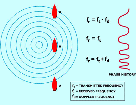
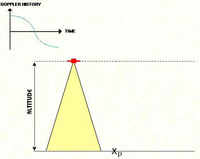
It is important to note that some details of the structure of the echoes produced by a given target change during the time the radar passes by. This change is explained also by the Doppler effect which among others is used to focus the signals in the azimuth processor. We will illustrate this point with an analogy.
Let us consider, as in the case of the second figure here, a plunger going up and down in the water, producing circles of radiating waves, each with a constant frequency fZ.
These waves travel at a known speed. The plunger is a source of waves analogous to those from a radar. We are interested in the appearance of this wave field at a certain distance.
Consider a boat is moving along the line. At position B, a passenger on the boat would count the same wave number as emitted, since he is moving neither toward nor away from the waves (source).
However, at position A, the boat is moving towards the waves and the passenger will count a higher number of waves: the travelling speed of the waves is slightly increased by the speed of the ship.
On the contrary, at position C, the boat is moving away from the buoy and the apparent frequency is lower: the waves are moving in the same direction as the boat.
Doppler frequency is the difference between received and emitted frequencies where the difference is caused by relative motion between the source and the observer.
Equivalently, the relative spacing between crests of the wave field could be recorded along the line AC, measured as if the wave field were motionless.
This leads to a phase model of the signals that is equivalent to the Doppler model.
During the movement of the boat from position A to position C, the recording by the observer of the number of waves would look like the curve at the right of the figure.
Instead of a plunger, let us now consider an aircraft emitting a radar signal. The boat corresponds to a target appearing to move through the antenna beam as the radar moves past.
The record of the signals backscattered by the target and received would be similar to the record of the passenger in the boat. Such a record is called the Doppler history (or phase history) of the returned signals.
When the target is entering the beam, the Doppler shift is positive because the source to target distance is decreasing. The phase history is then stored to be used during the SAR processing.
By the time the antenna is abeam relative to the target, the received frequency is nominal, with the Doppler frequency being zero. Late it decreases as the satellite moves away.
The phase history is then stored to be used during the SAR processing.
13. SAR processing
The objective of SAR processing is to reconstruct the imaged scene from the many pulses reflected by each single target, received by the antenna and registered in memory.
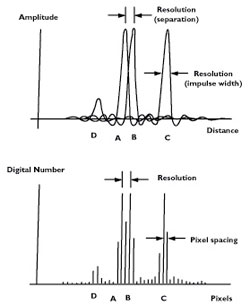
Resolution describes the minimal discernible spacing between two similar point responses (A and B), but often is applied to the width of one response (C). A weaker response (D) requires a larger separation for detection.
Pixels refer to the discrete sample positions used for digital imagery. There must be at least two pixels within a resolution distance.
SAR processing is a simple process although it requires much computation. It can be considered as a two-dimensional focussing operation.
The first of these is the relatively straightforward one of range focussing, requiring the de-chirping of the received echoes.
Azimuth focussing depends upon the Doppler histories produced by each point in the target field and is similar to the de-chirping operation used to focus in the range direction.
This is complicated however by the fact that these Doppler histories are range dependent, so azimuth compression must have the same range dependency.
It is necessary also to make various corrections to the data for sensor motion and Earth rotation for example, as well as for the changes in target range as the sensor flies past it.
It is important to note (see figure) that the pixel of the final SAR image does not have the same dimensions as the resolution cell during the data acquisition, due to the variation of range resolution with incidence angle. Thus it is necessary to perform a pixel resampling with a uniform grid.
Even more fundamental, at least two pixels are required to represent each resolution cell, which is a consequence of digital sampling rules. By convention, pixel spacing in SAR imagery is chosen to conform to standard map scales, hence must be a discrete multiple (or divisor) of 100 metres.
For example, ERS-1 data, having nominal resolution of 28 metres in range and azimuth, is delivered with 12.5 metre pixel spacings.
14. ERS SAR geometric configuration
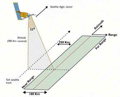
The spacecraft flew in its orbit and carried a SAR sensor which pointed perpendicular to the flight direction.
The projection of the orbit down to Earth is known as the ground track or subsatellite track. The area continuously imaged from the radar beam is called radar swath. Due to the look angle of about 23 degrees in the case of ERS, the imaged area is located some 250 km to the right of the subsatellite track. The radar swath itself is divided in a near range - the part closer to the ground track - and a far range.
In the SAR image, the direction of the satellite's movement is called azimuth direction, while the imaging direction is called range direction.
15. Slant range / ground range
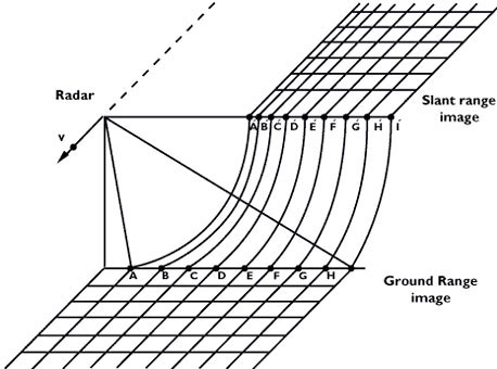
The figure shows two types of radar data display:
- slant range image, in which distances are measured between the antenna and the target
- ground range image, in which distances are measured between the platform ground track and the target, and placed in the correct position on the chosen reference plane
Slant range data is the natural result of radar range measurements. Transformation to ground range requires correction at each data point for local terrain slope and elevation.

This figure illustrates an example of SAR data using a Seasat scene of Geneva (Switzerland). The slant range image is displayed on the left of the screen, while the ground range image is on the right side.
The geometric distortions present on a radar image can be divided into:
- Range distortions: Radar measures slant ranges but, for an image to represent correctly the surface, it must be ground range corrected
- Elevation distortions: this occurs in those cases where points have an elevation different from the mean terrain elevation
16. Optical vs. microwave image geometry
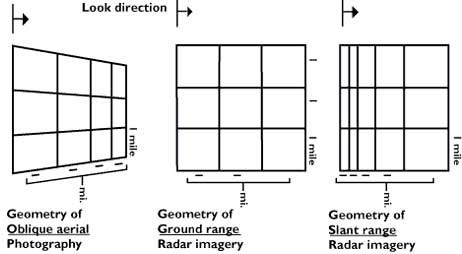
The figure presents a comparison between respective geometries of radar image and oblique aerial photos.
The reason for the major differences between the two image's geometry is that an optical sensor measures viewing angles, while a microwave imager determines distances.
17. Foreshortening
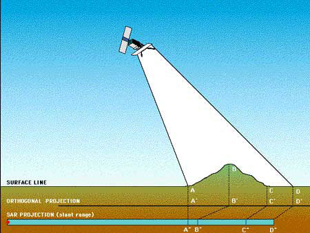
The most striking feature in SAR images is the "strange" geometry in range direction. This effect is caused by the SAR imaging principle: measuring signal travel time and not angles as optical systems do.
The time delay between the radar echoes received from two different points determines their distance in the image. Let us consider the mountain as sketched in the figure. Points A, B and C are equally spaced when vertically projected on the ground (as it is done in conventional cartography).
However, the distance between A'' and B'' is considerably shorter compared to B'' - C'', because the top of the mountain is relatively close to the SAR sensor.
Foreshortening is a dominant effect in SAR images of mountainous areas. Especially in the case of steep-looking spaceborne sensors, the across-track slant-range differences between two points located on foreslopes of mountains are smaller than they would be in flat areas.
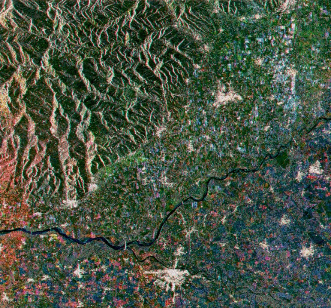
This effect results in an across-track compression of the radiometric information backscattered from foreslope areas (see example of ERS image to the left) which may be compensated during the geocoding process if a terrain model is available.
Foreshortening is obvious in mountaineous areas (top left corner), where the mountains seem to "lean" towards the sensor.
It is worth noting that shortening effects are still present on ellipsoid corrected data.
18. Layover
If, in the case of a very steep slope, targets in the valley have a larger slant range than related mountain tops, then the foreslope is "reversed" in the slant range image.
This phenomenon is called layover: the ordering of surface elements on the radar image is the reverse of the ordering on the ground. Generally, these layover zones, facing radar illumination, appear as bright features on the image due to the low incidence angle.
Ambiguity occurs between targets hit in the valley and in the foreland of the mountain, in case they have the same slant-range distance. For steep incidence angles this might also include targets on the backslope.
Geocoding can not resolve the ambiguities due to the representation of several points on the ground by one single point on the image; these zones also appear bright on the geocoded image.
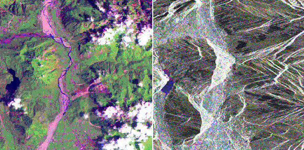
These images were acquired over a mountainous zone close to the city of Udine (I), by ERS-1 and Landsat-5 respectively.
The effect of layover is visible in the whole SAR image, in particular on the two mountains that are on the right of the lake. The height of the upper one (San Simeone) is about 1000 m above the valley bottom (1220 msl), while the height of the lower one (Brancot) is 1015 msl.
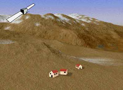
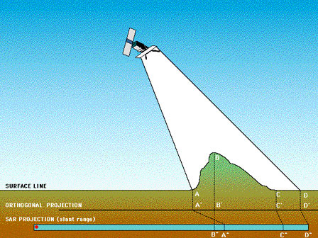
19. Shadow
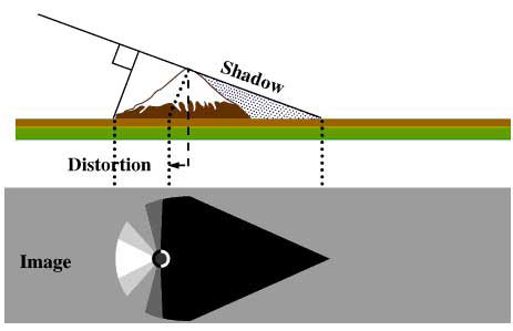
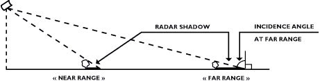
A slope away from the radar illumination with an angle that is steeper than the sensor depression angle provokes radar shadows.
It should be also noted that the radar shadows of two objects of the same height are longer in the far range than in the near range.
Shadow regions appear as dark (zero signal) with any changes due solely to system noise, sidelobes, and other effects normally of small importance.
Let us consider the mountain as sketched in the image. Points A, B, C and D are defining different parts of the target when vertically projected on the ground (the orthogonal projection, as it is done in conventional cartography). However, the segment between B and C is not giving any contribution in the slant range direction which is the SAR projection ( B'' - C'' ), due to the geometry of the mountain.
Note also the distance AB becoming orthogonal projected A' B'. In the slant-range projection this is A'' B'', much shorter, due to the foreshortening effect.

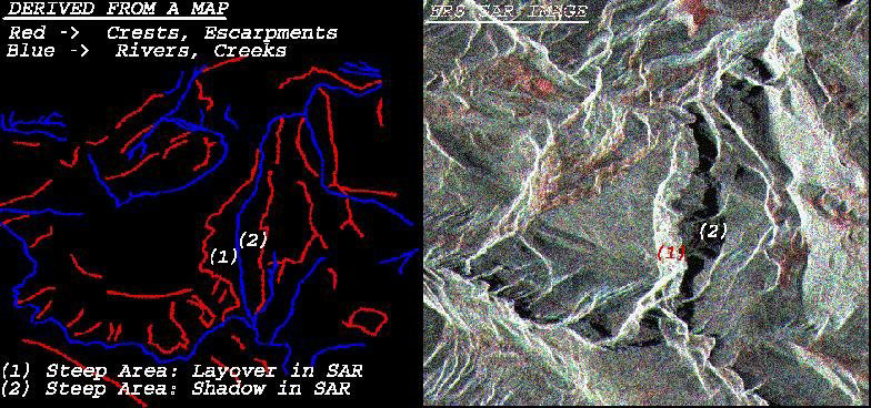
This multi-temporal (13-19-25/09/1991) SAR image has been acquired over the Cote D'Azur area (France). The Gran Canon du Verdon visible in the central part of the image has a very steep gorge that descends swiftly to the valley bottom, causing Radar shadow. This is shown by the dark zones in the central part of the image.
A map of the area may be useful to localise the feature.
20. Geometric effects for image interpretation
Based upon the previous considerations on SAR image geometry, the following remarks can be formulated in order to assist the interpreter:
- for regions of low relief, larger incidence angles give a slight enhancement to topographic features. So does very small incidence angles.
- for regions of high relief, layover is minimised and shadowing exaggerated by larger incidence angles. Smaller incidence angles are preferable to avoid shadowing.
- intermediate incidence angles correspond to low relief distortion and good detection of land (but not water) features.
- small incidence angles are necessary to give acceptable levels of backscattering from ocean surfaces.
- planimetric applications necessitate the use of ground range data, which usually requires use of digital elevation data and image transformation.
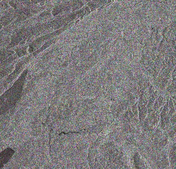
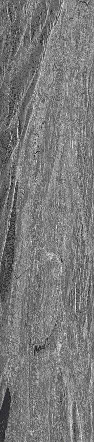
21. SAR image geocoding
The principle of side-looking SAR is measurement of the electromagnetic signal round trip time for the determination of slant ranges to objects and the strength of the returned signal. This principle causes several types of geometrical distortions.
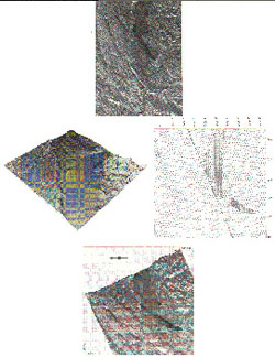
The upper part of the image shows an example of radar image with its characteristic slant range geometry. Severe distortions occur if pronounced terrain relief is present in the imaged zone.
The amount of distortion depends on the particular side-looking geometry and on the magnitude of the undulation of the terrain's surface.
The central part of the figure shows a digital elevation model of the zone that is used to create a grid map necessary to locate correctly the position of the pixels.
In many applications such as agriculture and vegetation mapping, the terrain-induced distortions degrade the usefulness of SAR images and in some cases may even prevent information extraction.
The lower part of the figure map represents the geometrically corrected image.
SAR data geocoding is a very important step for many users because SAR data should be geometrically correct in order to be compared or integrated with other types of data (satellite images, maps, etc.).
Geocoding an image consists of introducing spatial shifts on the original image in order to have a correspondance between the position of points on the final image and their location in a given cartographic projection.
Radiometric distortions also exist in connection with terrain relief and often cannot be completely corrected. In addition, resampling of the image can introduce radiometric errors.
For these reasons, the thematic user of the image needs information on what he should expect in terms of interpretability of geocoded images for a given thematic application.
A layover/shadowing mask and a local incidence angles map are both helpful for many applications.
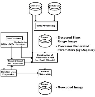
This figure illustrates a SAR geocoding system consisting of three data bases:
- Orbital parameters,
- Raw radar data,
- Geographic data base (Digital Terrain Model, Control Points and parameters of cartographic projection)
ERS-1 SAR looked at the Earth's surface with a 23° incidence angle. Due to this, images contained almost no shadow but may have contained a large amount of layover and foreshortening.
With the geocoded data, ERS-1 PAFs (Processing and Archiving Facilities) provide on request a data file indicating the layover and shadowed zones as well as the local incidence angle for each element of the picture.
This file is useful for the interpreter prior to thematic mapping. If a Digital Elevation Model is available, it may be possible to correct the terrain influence in SAR images.
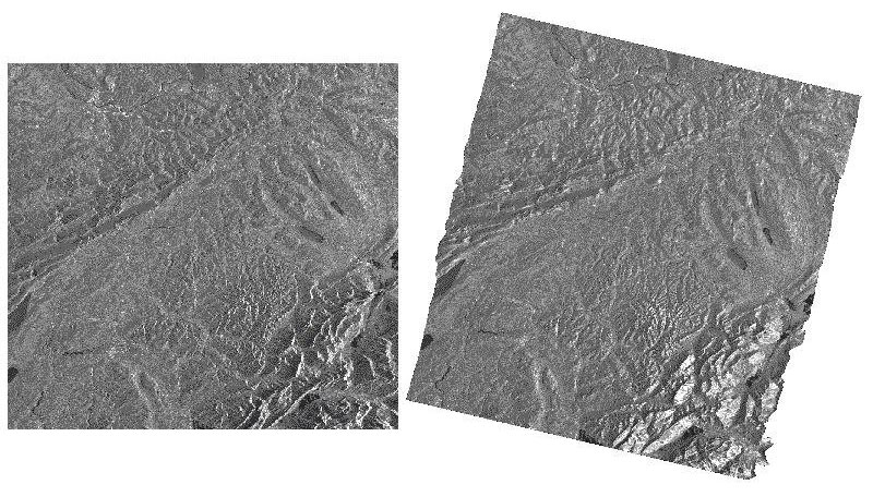
This figure illustrates an example of SAR data geocoding.
The reference scene (left of the screen) was acquired on 24 November 1991 over the north-western part of Switzerland and includes the city of Basel and the Rhine (top-left corner), the chain of the Jura mountains (northern part of the image), the Aare river crossing through the centre of the image with the capitol Berne near the lower left corner.
The southern part consists of lowland hills, the Napf area and the pre-alpine mountain chains.
The shores of the Lake of Lucerne (Vierwaldstätter See), in the south-east are not well defined due to wind-roughening effects.
The image presents strong geometric distortions which are no more visible in the corrected image displayed on the right.
22. Geocoding: Geometry
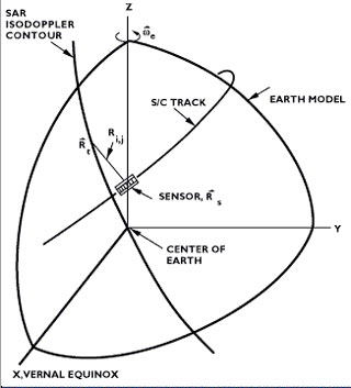
The location of the (i,j) pixel in a given image can be derived from knowledge of the sensor position and velocity. More precisely, the location of the antenna phase centre in an Earth referenced coordinate system is required.
The target location is determined by the simultaneous solution of three equations:
- Range equation
- Doppler equation
- Earth model equation
The figure shows the geocentrical coordinate system illustrating a graphical solution for the pixel location equations.
The range equation is given by

Where:
R s sensor position vector
R t target position vector
For a given cross-track pixel number j in the slant range image, the range to the j th pixel is
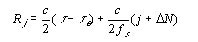
Where ΔN represents an initial offset in complex pixels (relative to the start of the sampling window) in the processed data set. This offset, which is nominally 0, is required for pixel location in sub-swath processing applications, or for a design where the processor steps into the data set an initial number of pixels to compensate for the range walk migration.
The Doppler equation is given by:
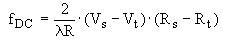
Where:
λ radar wavelength
fDC Doppler centroid frequency
Vs sensor (antenna phase centre) velocity
Vt target velocity
The target velocity can be determined from the target position by:
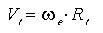
Where ωe is the Earth's rotational velocity vector. The Doppler centroid in the Doppler equation is the value of the used in the azimuth reference function to form the given pixel. An offset between the value of fDC in the reference function and the true causes the target to be displaced in azimuth according to
Where
ΔfDC is the difference between the true fDC and the reference fDC
fκ is the Doppler rate used in the reference function
and Vsw is the magnitude of the swath velocity
To compensate for this displacement, when performing the target location, the identical fDC used in the reference function to form the pixel should be used in the Doppler equation. The exception to this rule is if an ambiguous fDC is used in the reference function. That is, if the true fDC is offset from the reference fDC by more than +/- fp /2. In this case, the pixel shift will be according to the Doppler offset between the reference fDC and the Doppler centroid of the ambiguous Doppler spectrum, resulting in a pixel location error of
Where m is the number of PRFs the reference fDC is offset from its true value (i.e., the azimuth ambiguity number).
The third equation is the Earth model equation. An oblate ellipsoid can be used to model the Earth's shape as follows:
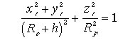
Where Re is the radius of the Earth at the equator, h is the local target elevation relative to the assumed model, and Rp, the polar radius, is given by

Where f is the flattening factor of the ellipsoid. If a topographic map of the area imaged is used to determine h, the Earth model parameters should match those used to produce the map. Otherwise, a mean sea level model can be used.
The target location as given by {xt, yt, zt} is determined from the simultaneous solution of the Range, Doppler and Earth model equations for the three unknown target position parameters.
This is illustrated in the figure; it shows the Earth (geoid) surface intersected by a plane whose position is given by the Doppler centroid equation. This intersection, a line of constant Doppler, is then intersected by the slant range vector at a given point, the target location. The left-right ambiguity is resolved by knowledge of the sensor's pointing direction.
The accuracy of this location procedure (assuming an ambiguous was not used in the processing) depends on the accuracy of the sensor position and velocity vectors, the measurement accuracy of the pulse delay time, and knowledge of the target height relative to the assumed Earth model.
The location does not require attitude sensor information. The cross-track target position is established by the sampling window, independent of the antenna footprint location (which does depend on the roll angle). Similarly, the azimuth squint angle, or aspect angle resulting from yaw and pitch of the platform, is determined by the Doppler centroid of the echo, which is estimated using a clutterlock technique.
Thus the SAR pixel location is inherently more accurate than that of optical sensors, since the attitude sensor calibration accuracy does not contribute to the image pixel location error.
23. Introduction to Interferometry
Accurate surface topographic data is required to investigate a wide variety of geophysical processes. An exciting and promising technique for the application of remote sensing data has emerged in recent years: Interferometric SAR, also called INSAR.
Using SAR interferometry, it is possible to produce directly from SAR image data detailed and accurate three-dimensional relief maps of the Earth's surface.
In addition, an extension of the basic technique, known as differential interferometry, allows detection of very-small (in the order of centimetres) movement of land surface features. Both of these possibilities open up many new potential application areas of spaceborne SAR data in the areas of cartography, volcanology, crustal dynamics, and the monitoring of land subsidence.
24. Concept

Interferometry allows the measurement of high resolution topographic profiles of terrain from multiple-pass SAR data sets. For the interferometric technique to be applicable, these data sets must be obtained when the sensor is in repeat orbit, such that the scene is viewed from almost the same aspect angle for each of the passes.
The figure shows the interferometric imaging geometry pointing out the two passes with range vectors r1 and r2 to the resolution element. The look angle of the radar is θ, the baseline B is tilted at an angle ξ measured relative to horizontal.
Each pixel of a SAR image contains information on both the intensity and phase of the received signal. The pixel intensity is related to the radar scattering properties of the surface, and the pixel phase to the satellite to ground path length, or distance.
Intensity images are the form of SAR data that is most frequently presented and probably most familiar to the public.
However, it is the phase information only (and not the image intensity) that is exploited by interferometric techniques, it contains informations about heights orthogonal to the SAR image plane.
An interferometer is a device that superimposes or mixes wave phenomena from two coherent sources.
First, the two SAR images are registered to each other to identify pixels corresponding to the same area of the Earth's surface.
Then, for each pixel, the phase values are subtracted to produce the phase difference image known as an interferogramme. This phase difference is a measure of the difference in path length from a given pixel to each antenna of the SAR interferometer.
The resulting interference effects are well-known both in optics (e.g., Newton's rings formed when a convex lens is placed on a plane surface) and sonics (e.g., beating formed by two similar frequency sound waves). Radar interferometry is the analogous phenomenon in the microwave region of the electromagnetic spectrum.
25. Method
The nearly exact repeat orbit allows formation of an interferometric baseline as shown in the figure. The ERS-1 sensor provided a platform to record SAR data which is useful for interferometry.
This exploitation of the orbit repeat feature is known as multi-pass INSAR.
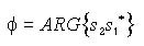
For a point target that is at (x, y, z), the phase difference f between the signal s1 and s2 received at r1 and r2 is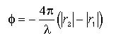
Where λ is the radar signal wavelength. The interferometric phase is obtained by complex correlation of the first complex SAR image, obtained during the first overpass, relative to the second image, belonging to the second pass, after precise co-registration.
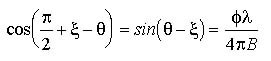
The interferometric phase can be used to determine the precise look angle Φ by first solving the cosine of the angle between the baseline vector and the look vector:
The height z at the location r1 is determined from:
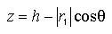
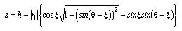
Where h is the altitude of the platform above the reference plane.
The phase in the interferogramme is known only modulo 2p, therefore it is necessary to determine the correct multiple of 2p to add to the phase to obtain consistent height estimates.
The correlation coefficient g of the complex backscatter intensities s1 and s2 at r1 and r2 is defined by:
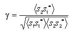
In the following we will call g the interferometric correlation. The correlation coefficient g in terms of the baseline correlation factor a is equal to
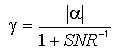
where the geometrical baseline correlation factor a is given by:
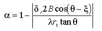
Where SNR is the signal to noise ratio, dr the slant range resolution, and alpha is the radar incidence angle.
The ERS-1 radar sensor has a slant range pixel spacing of 7.9 m, nominal incidence angle of 23 degrees, and nominal range of 853 Km to the center of the image swath.
For an 8 look image with a SNR of 20, the theoretical height resolution is better than 2.5 m for a wide range of correlation values y.
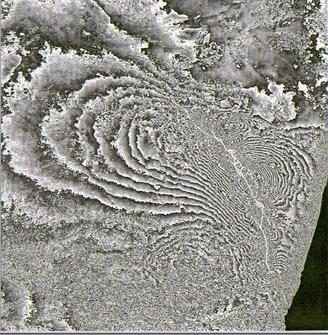
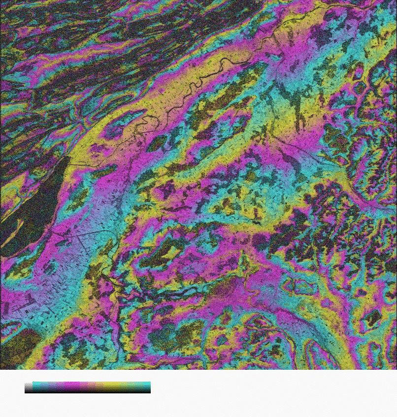
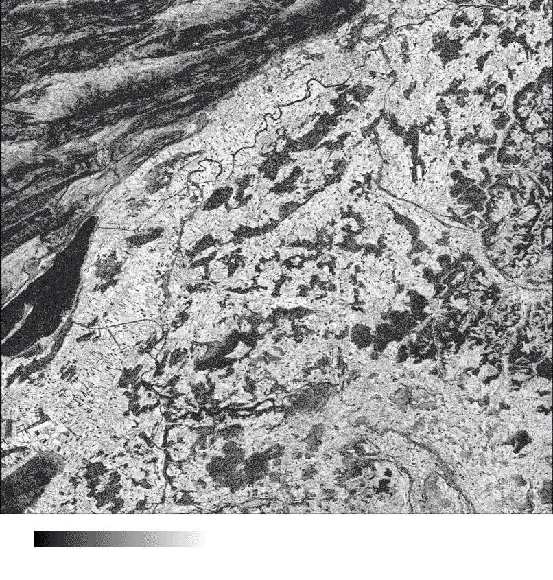
26. First ERS-1/ERS-2 tandem interferogram
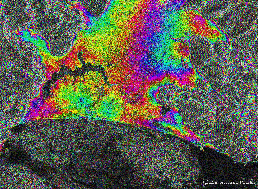
This image shows the interferometric phase obtained from the combination of an ERS-1 image taken on 1 May and the ERS-2 image taken exactly one day after, on 2 May. It demonstrates the feasibility of the tandem mission, which was conducted for ERS-1 and 2 between 1995 and 1996
An extract of the first ERS-2 image over the gulf of Gaeta in Central Italy was used in the generation of the coherence image. It contains an area of approximately 15 km by 20 km located in the far range of the original SAR image, just North of Gaeta.
The town of Terracina is located on the coast at the left of the interferogramme, while the village of Sperlonga can be seen on the coast on the right hand-side of the image.
In the plain in the middle of the image, one can see the lake of Fondi, which has taken its name from a town situated further into the plain.
The mountains surrounding the plain rise quite rapidly to heights between 800 metres and 1000 metres.
An interferogramme illustrates a technical complication associated with INSAR. The phase value (and hence phase differences) is not known absolutely, but is given in the range of 0-360° ; i.e., the phase is "wrapped" on to a fixed range of angle. The colour contours cycle through a colour wheel corresponds to a complete rotation of 360° in phase.
In order to compute terrain height and generate a DEM, the interferogramme has to be "unwrapped", i.e., the correct multiple of 360° added to phase value of each pixel. A number of algorithms exist to perform this task.
(Rocca, POLIMI, Milano)
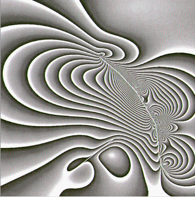
27. Naples (Italy)
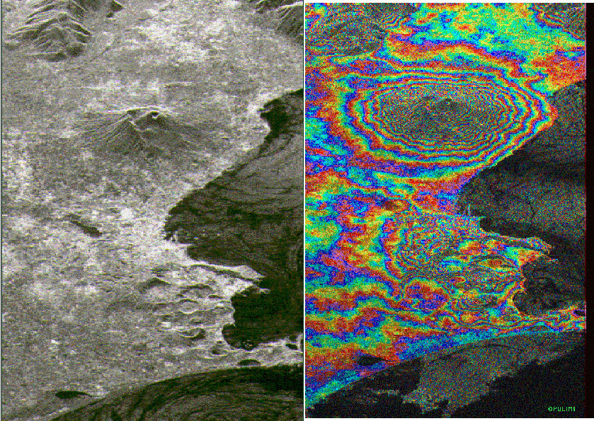
The image on the left side is an intensity image acquired over the Naples area (I) by ERS-1 in August 1991. The image has been "stretched" in the horizontal direction in order to show a better perspective view.
In the center of this image one can clearly distinguish the volcano Vesuvius. Below Vesuvius is the bay of Naples, and below Naples are the Caldera features of the Phlagrean Fields stretching to the coast. In the image, the white areas correspond to urban centres, and dark lines to motorways.
The figure on the right side shows an interferogramme of the same location.
The height contours of the Vesuvius are particularly striking. Note that no phase differences are given over the sea as the phase between passes is totally decorrelated due to the motion of the sea surface.
(Rocca, POLIMI, Milano)
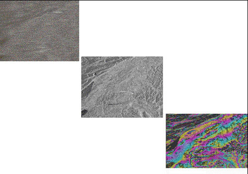
28. Coherence image of Bonn area (Germany)
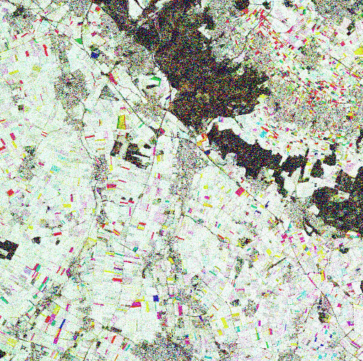
A series of ERS-1 SAR (Slant Range Complex) data sets of an area near Bonn, acquired during early spring 1994 has been analysed using interferometric methods. As the images were sampled at three days intervals, good phase-coherence between image-pairs could be expected. Images between 1 and 28 March were considered and totally 9 coherence images from different image-pairs were generated.
Agricultural fields appear in general quite bright in the coherence images, however some appear dark, indicating low coherence. In this cases, one can expect that coherence was lost due to farmer activities during the time between the two data acquisitions.
In order to verify this all coherence-images were provided to agricultural experts of the Bonn-University. They inquire about the farmers activities during March 1994, especially with respect to the dark-appearing fields in the coherence images. With respect to the relevant dates all fields were listed for type of crop and farmers activities.
In all cases a reason for the loss of coherence could be identified.
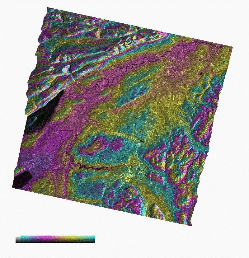
To demonstrate the farmers activities over a longer period a multi-temporal colour image was produced (see figure) choosing three of the nine coherence images, namely.
- 07/03/1994 - 10/03/1994 shown in red image channel
- 10/03/1994 - 13/03/1994 shown in green image channel
- 13/03/1994 - 16/03/1994 shown in blue image channel
All fields with equal grey-values in all three channels, i. e. with no change in coherence over the whole period from 07/03/1994 to 16/03/1993 appear not coloured, in black and white. The coloured fields result from different grey values in at least one of the three image planes (red or green or blue). The red fields have low coherence in the green and blue image plane, and hence no contribution from those to the colour-combination.
In fact the farmer ploughed the field twice, once between 13/03/1993 and 16/03/1993 and a second time between 16/03/1993 and 19/03/1993.
In yellow appear the fields with no coherence in the blue image plane, i. e. farming activities in this case must have taken place after the 13/03/1994.
In fact the field verification proved that farmer activities on these field were carried out between the 13 and 16 March. In the same manner all other colours could be explained.
Not only farmers activities, but also meteorological effects (rain, wind-fall), irrigation and of course all changes linked to vegetation growth can be reasons for de-correlation.
In our case, a loss of coherence especially related with growth can be neglected as vegetation canopy in March, if available at all is still very low and further, only a rather short time interval between two ERS-1 acquisition was considered.
(Wegmüller, Werner, Nuesch, RSL, Univ. Zurich)
29. Interferogram and DEM of Gennargentu (Italy)
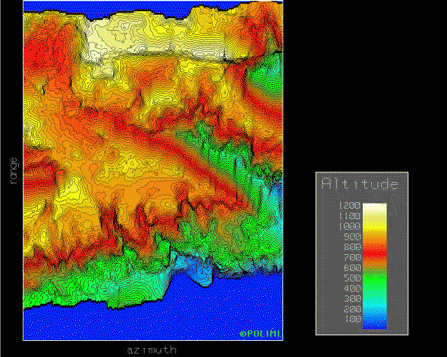

The figure shows an example of a DEM computed from ERS-1 SAR data gathered over the Gennargentu area (I) using the INSAR technique. The DEM has been derived from the interferogram of the same zone. The area consists of vegetated peaks rising rapidly from the coastline to a height of about 1200 m.
(Rocca, POLIMI, Milano)
30. Differential interferometry
Differential interferometry involves taking at least two images (with addition of DEM), normally three images, of the same ground area. Passes 1 and 2 are used to form an interferogram of the terrain topography using the basic interferometric technique. Similarly, passes 2 and 3 produce a further interferogram of the same area.
The two interferograms are then themselves differenced to reveal any changes that have occurred in the Earth's surface. Such changes could be the result of shifting geological faults or the buckling of the surface due to volcanic activity.
In principle, the ERS SAR was sensitive to changes of the Earth's surface topography on a scale comparable to the radar wavelength, i.e. 5.6 cmm.
31. The Bonn experiment
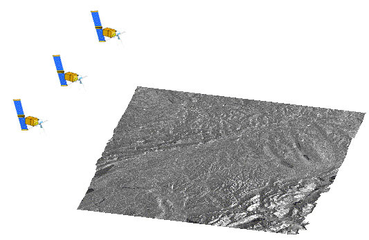
Taking advantage of the 3-day repeat orbit during the first ice phase of ERS-1, 19 corner reflectors (CR) were installed along an approximately straight line of 15 Km length in a relatively flat and homogeneous area west of Bonn.
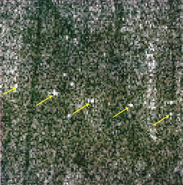
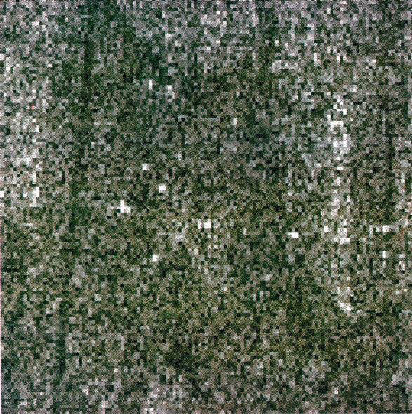
The ERS-1 SAR image shows the position of some corner reflectors placed in the area. The corner reflectors were constructed in such a way as to allow a vertical lifting.
From the 19 CRs only two had been lifted during the period in question. A vertical lifting of 1 cm was actually done at each, and this movement has been estimated using the SAR differential interferometry technique with an error of 1-2 mm.
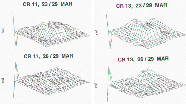
This figure shows the spatially averaged phase difference measured for the corner reflector N. 11 (left side) and N. 13 (right side).
The corner reflectors have been moved between the satellite passages of 23 March and the one of 26 March, and this is visible in the phase difference, comparing the phase differences between 23 and 29 and between 26 and 29 of March.
The experiment proved that the sensitivity of differential interferometry is in the sub-cm range, at least for point targets.
32. Landers Earthquake in South California
The Landers earthquake (south California) of 28 June 1992 (magnitude 7.3) presented a surface rupture over 75 km. It was followed three hours later by the Big Bear earthquake (magnitude 6.4). No surface rupture was reported for this later event.
From several images, acquired before and after the earthquake, a differential interferogram was computed (see figure), which clearly shows the seismic movements due to the earthquake. The banana-shaped fault is clearly visible. Each fringe corresponds to a co-seismic movement of 28.3 mm. The measured precision is 9 mm.
The differential interferogramme was compared with the effects of the movement predicted by an elastic dislocation model (computed by geophysicists of the French Groupe de Recherche an Géodésie Spatiale, GRGS), and the figure shows a very good correspondence between the modelled and the observed pattern of the fringes.
(Massonnet, CNES, Toulouse)
33. SAR interferometric products
ERS-1 quarter-scenes are presented as (raw) input, intermediate and possible final interferometric products.
The essential difference when compared to conventional detected SAR products (e.g. PRI) is that the phase resulting from the backscattered pulses of a target is preserved and used. Interferometric data applications use the phase change between acquisitions from the same orbital track. In principle, a minimum of one pair of data sets is necessary. Data application includes coherence maps, digital elevation models and mapping of small (centimetre-range) Earth movements.
The images presented in the following show parts of the Swiss Plateau crossed by the Aare river east to west.
In the examples below radar illumination is from the right and the flight direction is approximately north-south (descending pass). The data was acquired on 24 and 27 November 1991.
Animation of radar images:

Individual images used in animation:
- Raw Data
- Range Compressed Data
- One Look Complex Image
- One Look Complex Detected Image (I)
- One Look Complex Detected Image (II)
- Raw Interferogram
- Interferogram
- Coherence Image
- Digital Elevation Model
All image processing and text by: D. Small, E. Meier, D. Nuesch Remote Sensing Laboratories, Dept. of Geography, University of ZurichGeography, University of Zurich
34. Space, time and processing constraints
Space constraint: The interferometer baseline has to satisfy a condition determined by the radar characteristics and the imaging geometry. For ERS-1, the baseline (i.e., the component of the cross-track orbit separation perpendicular to the SAR slant range direction must not be greater than about 600 metres for the practical application of INSAR.
The complete set of ERS-1 restituted orbits that have been processed so far and an INSAR orbit listing has been produced at ESRIN. Using this listing, one can identify those repeated orbit acquisitions for which the orbits satisfy the INSAR baseline criterion.
Time constraint: Ideally, the two SAR images should be acquired simultaneously with a true interferometer. Therefore, in multi-pass INSAR, there should be no changes in surface conditions between the images which could effect the image phase values and lead to anomalous values of the computed terrain height. The effect of surface change is known as temporal de-correlation.
Research teams working with ERS-1 data are reporting good results with generally low values of temporal de-correlation for the 3-day repeat phases. In addition, INSAR has also been successful with ERS-1 data for some areas in the 35-day repeat phase.
Processing constraint: The SAR processor used to generate the imagery from raw satellite data must not introduce artefacts that corrupt the phase quality of the final image.
Currently, SAR processors within the ERS ground segment that have been validated for INSAR applications comprise:
- the Verification Mode Processor (VMP) used for calibration of the instrument, located at ESRIN;
- the precision processor located at the German PAF, from which users can order off-line SAR image products.
35. The radar equation
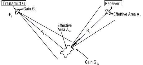
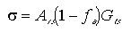
The fundamental relation between the characteristics of the radar, the target, and the received signal is called the radar equation. The geometry of scattering from an isolated radar target (scatterer) is shown in the figure, along with the parameters that are involved in the radar equation.
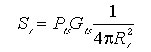
When a power Pt is transmitted by an antenna with gain Gt, the power per unit solid angle in the direction of the scatterer is Pt Gt, where the value of Gt in that direction is used. At the scatterer, (1)
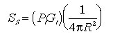
where Ss is the power density at the scatterer. The spreading loss

is the reduction in power density associated with spreading of the power over a sphere of radius R surrounding the antenna.
To obtain the total power intercepted by the scatterer, the power density must be multiplied by the effective receiving area of the scatterer: (2)

Note that the effective area Ars is not the actual area of the incident beam intercepted by the scatterer, but rather is the effective area; i.e., it is that area of the incident beam from which all power would be removed if one assumed that the power going through all the rest of the beam continued uninterrupted. The actual value of Ars depends on the effectiveness of the scatterer as a receiving antenna.
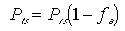
Some of the power received by the scatterer is absorbed in losses in the scatterer unless it is a perfect conductor or a perfect isolater; the rest is reradiated in various directions. The fraction absorbed is fa, so the fraction reradiated is 1- fa, and the total reradiated power is (3)
The conduction and displacement currents that flow in the scatterer result in reradiation that has a pattern (like an antenna pattern). Note that the effective receiving area of the scatterer is a function of its orientation relative to the incoming beam, so that Ars in the equation above is understood to apply only for the direction of the incoming beam.
The reradiation pattern may not be the same as the pattern of Ars, and the gain in the direction of the receiver is the relevant value in the reradiation pattern. Thus, (4)
where Pts is the total reradiated power, Gts is the gain of the scatterer in the direction of the receiver, and

is the spreading factor for the reradiation.
Note that a major difference between a communication link and radar scattering is that the communication link has only one spreading factor, whereas the radar has two. Thus, if Rr = Rt, the total distance is 2Rt; for a communication link with this distance, the spreading factor is only:
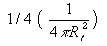
whereas for the radar it is:
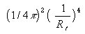
Hence, the spreading loss for a radar is much greater than for a communication link with the same total path length.
The power entering the receiver is (5)

where the area Ar is the effective aperture of the receiving antenna, not its actual area. Not only is this a function of direction, but it is also a function of the load impedance the receiver provided to the antenna; for example,Pr would have to be zero if the load were a short circuit or an open circuit.
The factors in the eq. 1 through the eq. 5 may be combined to obtain
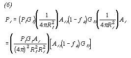
The factors associated with the scatterer are combined in the square brackets.
These factors are difficult to measure individually, and their relative contributions are uninteresting to one wishing to know the size of the received radar signal. Hence they are normally combined into one factor, the radar scattering cross section: (7)
The cross-section s is a function of the directions of the incident wave and the wave toward the receiver, as well as that of the scatterer shape and dielectric properties.
The final form of the radar equation is obtained by rewriting the eq. 6 using the definition of the eq. 7: (8)
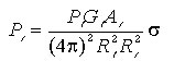
The most common situation is that for which receiving and transmitting locations are the same, so that the transmitter and receiver distances are the same. Almost as common is the use of the same antenna for transmitting and receiving, so the gains and effective apertures are the same, that is:
Rt= Rr =R
Gt= Gr =G
At= Ar =A
Since the effective area of an antenna is related to its gain by: (9)

we may rewrite the radar equation (eq. 8) as (10)
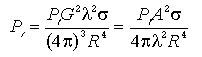
where two forms are given, one in terms of the antenna gain and the other in terms of the antenna area.
The radar equations (eq. 8 and eq. 10) are general equations for both point and area targets. That is, the scattering cross-section s is not defined in terms of any characteristic of a target type, but rather is the scattering cross-section of a particular target.
The form given in the equation 10 is for the so-called monostatic radar, and that in eq. 8 is for bistatic radar, although it also applies for monostatic radar when the conditions for R, G, A given above are satisfied.
36. Parameters affecting radar backscatter
Different surface features exhibit different scattering characteristics:
- Urban areas: very strong backscatter
- Forest: intermediate backscatter
- Calm water: smooth surface, low backscatter
- Rough sea: increased backscatter due to wind and current effects
The radar backscattering coefficient s 0 provided information about the imaged surface. It is a function of:
- Radar observation parameters:
(frequency f, polarisation p and incidence angle of the electromagnetic waves emitted); - Surface parameters:
(roughness, geometric shape and dielectric properties of the target).
Influence of frequency
The frequency of the incident radiation determines:
- the penetration depth of the waves for the target imaged;
- the relative roughness of the surface considered.
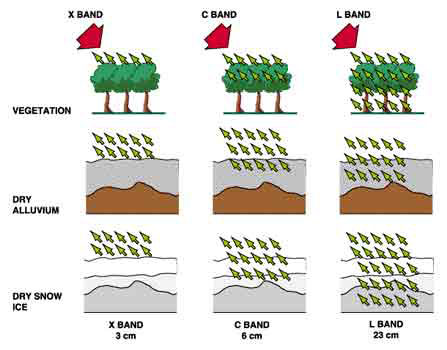
Penetration depth tends to be longer with longer wavelengths. If we consider the example of a forest, the radiation will only penetrate the first leaves on top of the trees if using the X-band (? = 3 cm). The information content of the image is related to the top layer and the crown of the trees. On the other hand, in the case of L-band (? = 23 cm), the radiation penetrates leaves and small branches; the information content of the image is then related to branches and eventually tree trunks.
The same phenomenon applies to various types of surfaces or targets (see the figure).
But it should be noted that:
- penetration depth is also related to the moisture of the target;
- microwaves do not penetrate water more than a few millimetres.
Influence of polarization
Polarization describes the orientation of the electric field component of an electromagnetic wave. Imaging radars can have different polarization configurations.
However, linear polarization configurations HH, VV, HV, VH are more commonly used. The first term corresponds to the polarization of the emitted radiation, the second term to the received radiation, so that XHV refers to X band, H transmit, and V receive for example.
In certain specific cases, polarization can provide information on different layers of the target, for example flooded vegetation. The penetration depth of the radar wave varies with the polarization chosen.
Polarization may provide information on the form and the orientation of small scattering elements that compose the surface or target.
More than one bounce of backscattering tends to depolarize the pulse, so that the cross polarized return in this case would be larger than with single bounce reflection.
Influence of roughness
Roughness is a relative concept depending upon wavelength and incidence angle.
A surface is considered "rough" if its surface structure has dimensions that are comparable to the incident wavelength.
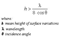
According to the Rayleigh criterion, a surface is considered smooth if:

and considered rough if:
An example of the effect of surface roughness can be observed in the zones of contact between land and water.
Inland water bodies tend to be relatively smooth, with most of the energy being reflected away from the radar and only a slight backscatter towards the radar.
On the contrary, land surfaces tend to have a higher roughness.
Water bodies generally have a dark tonality on radar images, except in the case of wind-stress or current that increase the water surface roughness, which provokes a high backscatter (see Bragg scattering, below).
In the microwave region, this difference between respective properties of land and water can be extremely useful for such applications as flood extent measurement or coastal zones erosion. This image illustrates the range of backscatter from water surfaces.
Influence of incidence angle
The incidence angle is defined by the angle between the perpendicular to the imaged surface and the direction of the incident radiation. For most natural targets, backscatter coefficient s 0 varies with the incidence angle.
Experimental work was conducted by Ulaby et al. (1978) using five soils with different surface roughness conditions but with similar moisture content. It appeared that, when using the L band (1.1 GHz), the backscatter of smooth fields was very sensitive to near nadir incidence angles; on the other hand, in the case of rough fields, the backscatter was almost independent of the incidence angle chosen.
Influence of moisture
The complex dielectric constant is a measure of the electric properties of surface materials. It consists of two parts (permittivity and conductivity) that are both highly dependent on the moisture content of the material considered.
In the microwave region, most natural materials have a dielectric constant between 3 and 8, in dry conditions. Water has a high dielectric constant (80), at least 10 times higher than for dry soil.
As a result, a change in moisture content generally provokes a significant change in the dielectric properties of natural materials; increasing moisture is associated with an increased radar reflectivity.
The electromagnetic wave penetration in an object is an inverse function of water content. In the specific case of vegetation, penetration depth depends on moisture, density and geometric structure of the plants (leaves, branches).
37. Bragg scattering
As the incidence angle of the ERS SAR is oblique (23) to the local mean angle of the ocean surface, there is almost no direct specular reflection except at very high sea states.
It is therefore assumed that at first approximation Bragg resonance is the primary mechanism for backscattering radar pulses.
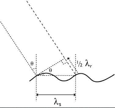
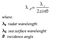
The Bragg equation defines the ocean wavelengths for Bragg scattering as a function of radar wavelength and incidence angle:
The short Bragg-scale waves are formed in response to wind stress. If the sea surface is rippled by a light breeze with no long waves present, the radar backscatter is due to the component of the wave spectrum which resonates with the radar wavelength.
The threshold windspeed value for the C-band waves is estimated to be at about 3.25 m/s at 10 metres above the surface. The Bragg resonant wave has its crest nominally at right angles to the range direction.
For surface waves with crests at an angle θ to the radar line-of-sight (see the figure on the left) the Bragg scattering criterion is
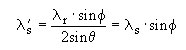
where: λ's is the wavelength of the surface waves propagating at angle θ to the radar line- of sight.
The SAR directly images the spatial distribution of the Bragg-scale waves. The spatial distribution may be affected by longer gravity waves, through tilt modulation, hydrodynamic modulation and velocity bunching.
Moreover, variable wind speed, changes in stratification in the atmospheric boundary layer, and variable currents associated with upper ocean circulation features such as fronts, eddies, internal waves and bottom topography effect the Bragg waves.
38. Radar image interpretation
Radar images have certain characteristics that are fundamentally different from images obtained by using optical sensors such as Landsat, SPOT or aerial photography. These specific characteristics are the consequence of the imaging radar technique, and are related to radiometry (speckle, texture or geometry).
During radar image analysis, the interpreter must keep in mind the fact that, even if the image is presented as an analog product on photographic paper, the radar "sees" the scene in a very different way from the human eye or from an optical sensor; the grey levels of the scene are related to the relative strength of the microwave energy backscattered by the landscape elements.
Shadows in radar image are related to the oblique incidence angle of microwave radiation emitted by the radar system and not to geometry of solar illumination. The false visual similarity between the two types of images usually leads to confusion for beginners in interpretation of radar images.
Elements of interpretation of radar imagery can be found in several publications for example, in "The use of Side-Looking Airborne Radar imagery for the production of a land use and vegetation study of Nigeria" (Allen, 1979).
Grey levels in a radar image are related to the microwave backscattering properties of the surface. The intensity of the backscattered signal varies according to roughness, dielectric properties and local slope. Thus the radar signal refers mainly to geometrical properties of the target.
In contrast, measurements in the visible/infrared region use optical sensors where target response is related to colours, chemical composition and temperature.
The following parameters are used during radar imagery interpretation:
- tone
- texture
- shape
- structure
- size
Several principles of photo-interpretation can be used for radar imagery interpretation and we can distinguish three steps:
- photo reading:
this corresponds to boundaries recognition on the basis of the previously listed parameters. - photo analysis:
this corresponds to the recognition of what is within the boundaries previously identified. - deductive interpretation of image:
At this stage, the interpreter uses all his thematic knowledge and experience to interpret the data.
Before describing texture, we can propose the following definitions:
- Tone
Radar imagery tone can be defined as the average intensity of the backscattered signal. High intensity returns appear as light tones on a positive image, while low signal returns appear as dark tones on the imagery. - Shape
It can be defined as spatial form with respect to a relative constant contour or periphery, or more simply the object's outline. Some features (streets, bridges, airports...) can be distinguished by their shape. It should be noted that the shape is as seen by the oblique illumination: slant range distance of the radar. - Structure
The spatial arrangement of features throughout a region with recurring configuration. - Size
The size of an object may be used as a qualitative recognition element on radar imagery. The size of known features on the imagery provided a relative evaluation of scale and dimensions of other terrain features.
39. Image interpretation: Tone
Different surface features exhibit different scattering characteristics:
- Urban areas: very strong backscatter
- Forest: medium backscatter
- Calm water: smooth surface, low backscatter
- Rough sea: increased backscatter due to wind and current effects
The average backscattering coefficient s 0 differs according to the types of surface, so it may be reasonably expected that surfaces with different values of s 0 would produce different grey levels in the image.
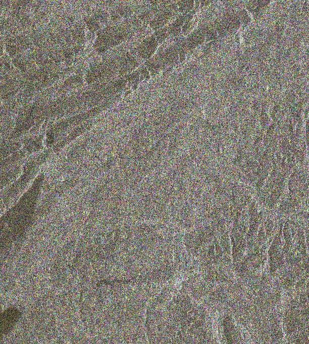
40. Image interpretation: Speckle

A detailed analysis of the radar image shows that even for a single surface type, important grey level variations may occur between adjacent resolution cells. These variations create a grainy texture, characteristic of radar images. This effect, caused by the coherent radiation used by radar systems, is called speckle. It happens because each resolution cell associated with an extended target contains several scattering centres whose elementary returns, by positive or negative interference, originate light or dark image brightness. This creates a "salt and pepper" appearance.
An example of speckle is shown in the figure.
The SAR scene acquired on 21/4/1994 over Tiber Valley (I) shows some agricultural fields located along the Tiber River north to Rome, in the central part of Italy.
The homogeneous patches representing the fields have high variability in backscattering due to the speckle noise. This results in a grainy image, which renders difficult the interpretation of the main features of the surface imaged by the SAR.
Speckle is a system phenomenon and is not the result of spatial variation of average reflectivity of the radar illuminated surface. For a high resolution radar, there may be useful scene texture which differs from the speckle.
This is the case for example in forested zones where the combined effects of radar illumination and tree shadowing create a rougher texture granularity than the speckle. In this case, there exists a spatial variability of the physical reflectivity of the illuminated zone. In a radar image we may find:
- zones where the only image texture is related to speckle that we may call regions "without texture" (extended homogeneous target)
- zones "with texture" that have spatial variations in scene reflectivity in addition to speckle
Thus, in the case of "no texture" zones, it becomes possible to study the statistical distribution of the backscattered radar signal, which helps to estimate certain radar characteristics.
Speckle can be reduced by two methods:
SAR image multi-look processing
Independent measurements of the same target can be averaged in order to smooth out the speckle. Actually, it is obtained by splitting the synthetic aperture into smaller sub-apertures, the so called "looks", each separately processed and then averaged.
The different looks are averaged to reduce the grey level random variations provoked by speckle. For N statistically independent (non-overlapping) data sectors, the speckle variance is reduced by a factor of N. Likewise, the resolution is degraded by a factor of N.
In such a way, we can for example have 8-look images. A compromise has to be found between desired spatial resolution and an acceptable level of speckle.
Filtering techniques
When the finest resolution is required, moving window filters are used. A moving window filter changes the intensity of the central pixel depending on the intensities of all the pixels within the window. Different algorithms have been proposed to properly shape the impulse response of the filter within the window.
In both cases speckle is reduced at the expenses of the spatial resolution.
41. Image interpretation: Speckle filters
We can consider that an extended area is characterised by:
- the radar backscattering coefficient s ° (radiometric information)
- spatial variability (textural information)
The presence of speckle reduces the separability of the various land use classes, based on radiometry and texture. It is thus important to treat speckle so as to improve the possibility of separation, but with minimal loss of information.
If we take the example of homogeneous areas such as agricultural zones with a defined field pattern, the filters to be used must preserve the average backscattering value, and maintain sharp edges between adjacent fields.
In the case of textured areas, such as forest for example, the filters should also preserve the spatial variability (textural information) relating to the scene.
The figure provides an example of simple filter. On the left part of the screen is displayed the speckled SAR image, and on the right part a filtered version of the same image. The filter applied in this case is the Mean filter which substitutes the central pixel with the mean value within the window. It results in a less noisy, but blurred, image.
More complex filters try to make some hypotheses on the noise statistic. The Frost filter models the signal as a slow varying function representing the texture of the scene multiplied by a gaussian distributed noise. The result of the filtering is shown on the right part of the image, while on the left part it is possible to observe the original SAR image. Filtering with this technique results in a less noisy image, better preserving the actual texture of the scene.
A more refined technique of speckle filtering is performed with the MAP Gamma filter. This filter models the distribution of the texture as a Gamma distribution and applies a maximum likelihood estimation to retrieve the detected intensity.
A separate routine allows to detect edges and lines. The result of the filtering is showed on the right part of the figure, together with the unfiltered SAR image (left side), and it is particularly useful for classification purposes.
42. Temporal averaging
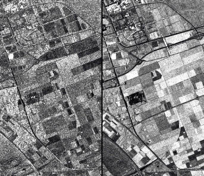
Another approach in image filtering is presented here. This simple technique can be called temporal averaging. It has the advantage of reducing the speckle without loosing spatial resolution: the contrary is the case of multilooking.
A subscene from Flevoland/The Netherlands has been used. The ERS SAR image to the left is the acquisition of 23 May 1993. To the right is a pixel by pixel averaged image of a data set consisting of 11 superimposed SAR scenes of that year (one each month with the exception of July).
As a result, fields become more homogeneous and their boundaries are better defined. Point-targets are enhanced, rendering the image much more focused.
Such simple techniques can be applied to improve spatial resolution, in the case high resolution optical data are not available or can not be afforded. It is required as input for the extraction of field boundaries in order to segment SAR images. The scope is to extract mean-values and other statistical parameters of each field of individual scenes for subsequent classification.
A more general application is its use in mapping, for the detection and interpretation of smaller objects.
(M. Mangolini, formerly of ESA/ESRIN)
43. Texture and image analysis
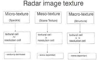
The concept of texture is discussed by Laur (1989). Before describing the specificity of radar image texture, it is necessary to define the concept of textural element, i.e. the texture elementary unit, smallest homogeneous element of the same radiometry constituting the texture.
In principle, the texture of a radar image can be described by considering Macro-texture, Meso-texture and Micro-texture. Let us consider the following example to illustrate these three texture categories.
An observer flies with a sensor above a wooded area, high enough not to recognise single leaves but low enough to distinguish clearly tree crowns.
First, he identifies the different stands; these might be oaks, pines, beeches, etc.
The different stands define the macrotexture or structure of the scene. The crowns are the key element to identify the content of a stand and define the mesotexture, a crown being a texture unit in this example.
The grey level of each resolution cell depends on the quantity and orientation of the leaves that scatter the incoming light. Horizontal leaves reflect much more than vertical ones.
This difference between resolution cells of the same class appears in the image as microtexture, called speckle or image noise on a radar image.
The texture of a radar image can be divided into three components:
Micro-texture, i.e. speckle, that appears as grains of the same size as or larger than the resolution cell, and having a random brightness. This texture is inherent to the radar system; it does not correspond to a real variation from one resolution cell to another.
Thus, speckle is essentially an image texture arising from the system, and not from the scene. Speckle degrades image readibility. However, despite this major disadvantage, speckle may be statistically characterised. This point may be exploited by speckle filtering methods.
Meso-texture or "scene texture" is the natural variation of average radar backscatter on a scale of several resolution cells or more. Taking forests as an example, the high backscatter from the part of the tree facing the radar appears near the shadow of the opposed part of the tree away from the radar.
The result is a grainy texture whose elementary unit covers several resolution cells (depending on the spatial resolution of the system). It is this component of image texture that is most useful in the interpretation of the radar image.
Macro-texture corresponds to variations in radar brightness that extend over many resolution cells. It can be, for example, field boundaries, forest shadows, roads or geologic lineaments.
The structure parameter is extremely important for radar imagery interpretation, especially in geology and oceanography. It is generally assessed using edge or other pattern detection techniques.
Based on this discussion, some observations may be made:
- Speckle is superimposed on scene texture and structure, creating problems during textural analysis or edge detection of imagery. In general, speckle is a product function: it is multiplicative, not additive although speckle modelling for scenes of rapidly changing contrast is more complex.
- Tone, i.e. average value of the mean cross section s °, is a local concept. It is the spatial variation of tone that provides "texture".
- Texture is related to the spatial distribution of resolution cells and depends on the scene, not on the system. Nevertheless, radiometric quality must be relatively constant in the samples where textural measurements are performed.
- Texture and structure are limited by the spatial resolution.
- Any post-processing of a SAR image (filtering, texture analysis) should be performed on radiometrically original images (slant range). Ground range images are resampled and thus may be radiometrically distorted.
44. Classification of ERS-1 SAR images with Neural Networks
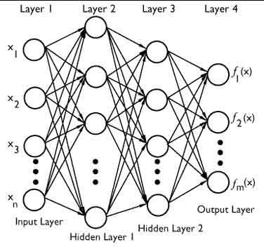

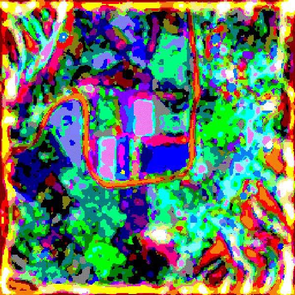
SAR technique offers a range of valued remote sensing products. Among them, SAR images that are plentiful of information about the orphology and the orography of the surface, and can be acquired at any time and with any weather.
The drawback is that these images are affected by a tedious multiplicative noise that strongly inhibits the possibility of applying automatic processing procedures to extract the desired information from them, and in particular to perform automatic classification.
The most surprising phenomena is that a human observer has little difficulty in recognising fields, structures and objects on a SAR image, even with high level of noise, with results close to the ones obtainable from inspecting optical images.
The explanation resides in our ability to extrapolate the shapes and the features of the image out of the noise, due to the very-high level activities in the brain, able to perform a hard job of pattern matching on a wide range of patterns.
The "things" we see in the image are implicitly compared with the patterns we accumulated in mind during our individual experience, and sometimes we see different things depending on how our attention is biased.
The classification of images could be roughly divided into classification of pixels on the basis of their spectral components, and classification of areas and details on the basis of their morphology and shape.
For both of them Neural Networks (NNs) offer a suitable technique, flexible and powerful, due to the capability of NNs to learn from examples and to accumulate, during the learning phase, in their artificial synapsis (the long term memory) the "know-how" to give the most likely answer to the current input.
A Neural Network is a set of processing units (the neurons) defined by an Input Function, a Transfer Function and an Output Function. The neurons communicate by means of Weighted Connections whose values are changed by the learning activities.
The behaviour of a NN depends on the Input, Transfer and Output Functions of each neuron, on the weights of the connections and also on the topology of the network.
In some topologies the NNs are organised in "layers" of neurons. When the data in the network flow from the input layer to the output layer crossing the intermediate layers (called hidden layers) without feedbacks, then the network is called "feed forward".
The figure shows the topology of a multi-layer feed-forward artificial Neural Network.
When in the network there exist layers with reciprocal connections, then the network is called "recurrent". A feed forward network with n input neurons and m output neurons can be trained with a set of input vectors xi of n components and a corresponding set of desired output vectors fi(x1 , x2 ...xm) of m components, so that it learns to behave as a function Y=f(X).
Once the network is trained, it will associate to the generic vector X, the corresponding vector Y, according to the behaviour learned from the training set. Such feature is useful when a set of X and Y data are available (training set) but it is hard to define analytically the function f.
In remote sensing this is the usual situation, where X are the spectral contents of the pixel and Y are the corresponding ground truths; such a training set could be derived from a test site, to train a network, and then the network could be used to classify a whole set of images. The availability of the desired outputs, corresponding to a set of input data, allows the use of Supervised Learning algorithms to train the network. When there is the need to classify some images but a set of input-output data is not available, then the NN technique is still applicable. Now is up to the NN to "decide" the best output corresponding to the current input.
Once again, before the NN can perform the classification, it has to be trained, but now with an Unsupervised Learning algorithm and a training set containing only input data. There are a number of NN typologies, and corresponding learning algorithms, suitable for Unsupervised classification.
Among them the Learning Vector Quantization (LVQ) family and the derived Kohonen's Maps, emerge as the best trade-off between computation resources needed (memory and CPU time) and minimisation of the number of misclassified input vectors. According to benchmarks, a LVQ classifier tested on the "satimage" database presents a percentage of misclassified input vectors below 12%.
It has to be remarked that a sort of preprocessing is needed before using any kind of classifier on SAR images. The morphology informations embedded in the image, along with local statistics (mean and variance), could be used to attribute an artificial spectrum to the pixels of a single SAR image. Also in case of multi-temporal images a lowering of the noise and an extraction of morphological features are helpful to perform reliable classification.
The results of this approach are shown in these two figures. The first image is a multi-temporal ERS-1 SAR scene (FDC, April, May, July 1992, Tiber Valley north of Rome), and the second figure shows an unsupervised classification obtained by a NN (3-dimensional Kohonen's Map) after features extraction and statistics computation.
In some aspects the NNs behaviour looks very close to that of a photo-interpreter: its ability grows with the practice, and early learnings could be confirmed or discarded on the basis of more and more examples. As for human operators, a NN could be specialised on a specific typology of images, but the comparison between the human behaviour and a NN stops here!
Nevertheless, this technology is going to be applied even more in real problems and applications, emerging from research environments, and today appears to be one of the most viable approaches in the automatisation of complex tasks solution.
45. Data reduction: 16 to 8 bit, blockaverage vs incrementing

The figure to the left of the screen was obtained from the full resolution image by means of a block averaging of 16x16 pixels moving window. The average value of each window is written to a new image file which dimension is reduced by 16 times in lines and columns. This is a conventional way to obtain a good quality Quick-Look images starting from a full-resolution image.
On the right part of the screen an 8 bit version of the full resolution image is shown. It has been obtained merely sampling the full image using a step increment of 16 pixels. The process results in a final image that has the same size of the image displayed on the left.
For practical reasons also a 16 to 8 bit conversion is done. Original statistics are conserved best when applying a square root to the original 16 bit data. Especially the information from point targets (strong scattering) are retained.
If mainly distributed targets (e.g. agriculture) are evaluated, a simple division (e.g. by four) is applied. This procedure clips all values greater than 1020, in the presented cases a division by four has been performed.
The dimension of the 16 bit full-resolution image which was initially about 128 Mbytes has now been reduced by a factor 256 for the processing and by a factor 2 for the reduction from 16 to 8 bit. This results in a final size for the image of about 250 Kbytes.
The main difference characterising the two images is in the amount of noise. In the right one it is possible to note that the increase of noise due to the resampling process masks the smaller features of the image and part of the SAR information is lost. In this image, even if the effect of the rain cells is still visible in the central part of the figure, most of the small features such as the presence of ships or the local effects of the wind on the sea surface are lost. Note also that the urban environment (bright part), in the upper part of the left figure, appears, in the right image, defocused because of the noise.